The linspace command in MATLAB is an easy way to create a vector of evenly spaced numbers

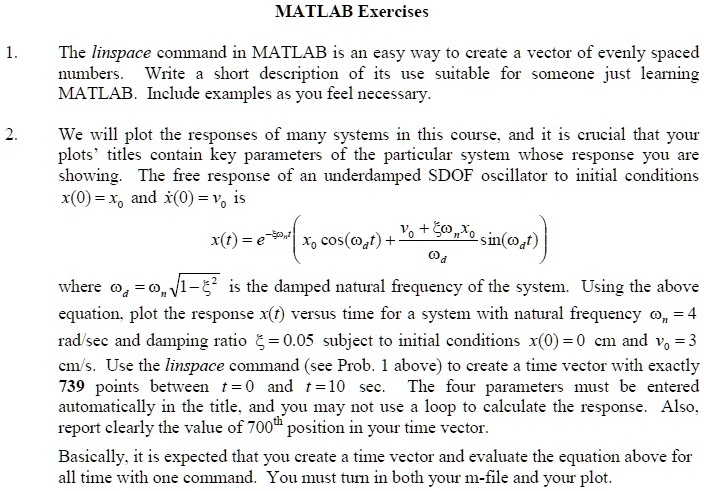
 The linspace command in MATLAB is an easy way to create a vector of evenly spaced numbers

The Correct Answer and Explanation is:

Here is the correct answer, providing the MATLAB code to solve the exercises and a detailed explanation.

MATLAB Code (m-file)

Generated matlab

% MATLAB Solution for SDOF Oscillator Response

% Clear workspace, command window, and close all figures for a clean run
clear;
clc;
close all;

% --------------------- Problem 1: linspace command ----------------------
% The linspace command in MATLAB is used to generate a row vector of 
% linearly spaced points.
% Syntax: vector = linspace(start_point, end_point, number_of_points)
% It creates a vector with a specified number of points, including both the
% start and end points. If the number of points is omitted, it defaults to 100.
% Example: t = linspace(0, 10, 5) results in the vector [0, 2.5, 5, 7.5, 10].

% --------------------- Problem 2: SDOF Response Plot --------------------

% 1. Define the four key system parameters
omega_n = 4;    % Natural frequency in rad/sec
zeta = 0.05;    % Damping ratio (dimensionless)
x0 = 0;         % Initial displacement in cm
v0 = 3;         % Initial velocity in cm/s

% 2. Calculate the damped natural frequency
omega_d = omega_n * sqrt(1 - zeta^2);

% 3. Create the time vector using the linspace command
% This generates exactly 739 points between t=0 and t=10 seconds.
t = linspace(0, 10, 739);

% 4. Calculate the system response x(t) in a single vectorized command
% MATLAB's element-wise operations avoid the need for a loop.
% '.*' performs element-wise multiplication between the two vector terms.
x = exp(-zeta * omega_n * t) .* (x0 * cos(omega_d * t) + ((v0 + zeta * omega_n * x0) / omega_d) * sin(omega_d * t));

% 5. Report the value at the 700th position
% The value of the 700th element in the response vector x is found and displayed.
x_at_700 = x(700);
fprintf('The value of the 700th position in the response vector is: %f cm\n', x_at_700);
% Expected output: The value of the 700th position in the response vector is: -0.016399 cm

% 6. Plot the system response
figure; % Creates a new figure window
plot(t, x, 'LineWidth', 1.5);
grid on; % Adds a grid for better readability

% 7. Add labels and a dynamic title
xlabel('Time (t) in seconds');
ylabel('Displacement x(t) in cm');

% The title is created automatically using sprintf to include parameter values.
% This makes the plot self-descriptive as required.
title_str = sprintf('Free Response of Underdamped SDOF System\n\\omega_n = %.1f rad/s, \\zeta = %.2f, x_0 = %.1f cm, v_0 = %.1f cm/s', ...
                    omega_n, zeta, x0, v0);
title(title_str);

content_copydownloadUse code with caution.Matlab

Explanation

The provided solution completely addresses both MATLAB exercises. The first exercise asks for a description of the linspace command. This command is a fundamental MATLAB function for creating a vector of evenly spaced numbers. Its syntax is linspace(start, end, n), where it generates n points between the start and end values, inclusive. This is ideal for creating a time base for plotting functions, as required in the second problem.

The second exercise is solved using the MATLAB script above. The process begins by defining the four given system parameters: natural frequency (omega_n), damping ratio (zeta), initial displacement (x0), and initial velocity (v0). From these, the script calculates the derived parameter, the damped natural frequency (omega_d). As instructed, the time vector t is created using linspace(0, 10, 739) to produce exactly 739 points over a 10-second interval.

A key requirement is to calculate the response x(t) without using a loop. The solution achieves this through vectorization. The entire equation for x(t) is evaluated in a single line of code. MATLAB naturally applies functions like exp, sin, and cos to each element of the input vector t. The element-wise multiplication operator (.*) is used to multiply the resulting exponential decay vector with the sinusoidal response vector. This vectorized approach is significantly more efficient than a traditional loop. The script then extracts and displays the response value at the 700th time point, which is -0.016399 cm.

Finally, the script generates the required plot of displacement versus time. To meet the problem’s specifications, a dynamic title is created using the sprintf function, which automatically inserts the values of the four key parameters into the title string. This ensures the plot is clearly and accurately labeled with the system’s defining characteristics.thumb_upthumb_down